Making processors fast again

This post should preferrably (but not necessarily) be read in continuation to the previous post titled Fueling high performance in computing.

Buying performance

Programming has always thrived on the use of abstractions. Someone who builds websites typically doesn’t (and shouldn’t) need to know about the changes in each of the generations of processor chips. Furthermore, just like buying more storage means you can save more data, buying a newer processor should mean you can run a single computation faster (without code re-write, assuming it is already compute-heavy). Typically, a processor executes instructions in locksteps (or clock ticks). Increasing the speed of a processor (till the 80s) meant reducing this lockstep duration. This would hence make programs run faster without any code rewrite.

Trouble in paradise

This wonderful cycle lost steam when it became extremely difficult to scale the clock speed any more. The problem was that the power used (and the heat produced) by these processors started increasing faster than their performance.

Regardless, computer architects soon found a workaround to keep making processors faster. To understand the solution, let us take a look at the brief organisation of a processor:

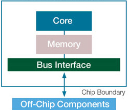
A “Core” as shown in the image is the fundamental unit that does the required arithmetic computation(s). The aforementioned clock speed influences the speed of this core and hence the processor as a whole.

A diabolical hack

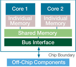
Coming back to the problem, it was clear that one core could not get any faster. So, why not just add more cores to a single processors?

Earlier, if you would have increased the clock speed of a single core by \(2X\), you would have needed (approximately) \(4X\) power to run it. But instead, to run two cores you needed just \(2X\) power. This hence gave some room to keep scaling the performance.

With the advent of parallel processors however, it was suddenly impossible to simply “buy” performance. This architectural change had unprecedented far-reaching implications for everyone. The newfound concurrency was like quantum uncertainty to the deterministic universe of programs. Several new bugs came up due to parallelism in programs. You see, these cores could be given conflicting tasks to do, and any kind of safety checks at run-time would reduce performance. Testing and debugging also got (and still is!) a whole lot trickier.

However, this was the easy part. You see, even theoretical computer science had to play catch-up with this architectural change. Regardless of what the local Apple “Genius” says, it is a fallacy to always expect linear scaling–with respect to the number of cores–for any given algorithm.

Earlier, theoretical analysis of an algorithm was done with the assumption that a hardware change will affect all algorithms equally. Suddenly, this was not true! Some algorithms could work better on parallel processors than others. I’ll try to explain this with the following example.

A game of kingdoms

We have a grid of 5 x 5. Imagine that each cell in the grid is an independent kingdom. You are a conqueror, and want to rule the 25 kingdoms and sit on the beyond-iron throne (a sustainable replacement for iron, made out of leaves and twigs, but looks just like iron).

However, let’s imagine you are working alone. You can only capture one kingdom per day (no one can defeat you), and hence grow your territory. A territory is just a group of kingdoms that share a wall with each other (adjacent cells) and are controlled by the same king.

So, how many days would it take you for world domination?

Well, obviously 25. As shown below, you can start at the top left corner and conquer kingdoms as you go left to right and top to bottom. Or you could start at the center and work your way outwards. All the possible sequences of moves are equivalent in this case.

1	2	3	4	5
6	7	8	9	10
11	12	13	14	15
16	17	18	19	20
21	22	23	24	25

In an alternate scenario, let’s imagine you are the leader of the unsullied. You basically command an infinite set of people, all of whom will fight for you, and needless to say, always win.

But here’s the catch. On each day, you can either choose to (all by yourself) conquer a new kingdom that does not share a wall with your current territory (and thereby making a new territory with a single kingdom), OR, you can use your men to annex all kingdoms that are adjacent to any one of your current territory(ies).

For example:

Let’s say, at the end of a day you have two territories, one on the top left end of the grid and one at the bottom right end as shown:

X	X
X
			X	X
				X

The next day, you can either grow the territory at the bottom right end, or at the top left end or venture out and make a new territory with a single kingdom. The three possibilities are shown in the same order:

X	X
X
			X	X
		X	X	X
			X	X

X	X	X
X	X
X
			X	X
				X

X	X
X
			X	X
X				X

Now, what is the fastest way to rule the 25 kingdoms? Well, just take the center kingdom and keep growing this territory every day. Easy.

5	4	3	4	5
4	3	2	3	4
3	2	1	2	3
4	3	2	3	4
5	4	3	4	5

The above grid shows you at which day you will get the respective kingdoms. On day 5, you can sit on the beyond-iron throne!

However, not all strategies are so fast. Consider a bad start near a corner, this is what will happen:

3	2	3	4	5
2	1	2	3	4
3	2	3	4	5
4	3	4	5	6
5	4	5	6	7

In this case, you will finish on the 7th day. Needless to say, both of these strategies were equal if you were fighting alone.

This example shows that some algorithms make better use of parallel hardware than others! This is because parallelising an algorithm might have some inherent limitations. Some computations can not be done in parallel with each other. Hence, some parts of the algorithm scale up very well while others don’t scale at all.

In the sequential world the run-time was dictated primarily by how many computations were being performed, but in the parallel world it is also greatly influenced by how interdependent these computations are.

Some generic theoretical analysis had previously been done for useful problems. For such a problem (for eg: sorting) it was shown that any algorithm that solves it correctly, has to do at least a certain number of computations. This was pretty useful. If you came up with an algorithm that is at this lower bound, you knew that there was no more room to optimise it.

With parallel processors, this was not so black and white anymore. The architects had just opened up a new pandora’s box of scalability. Not all algorithms that were declared time-optimal could scale equally well. It actually gets worse. Some sub-optimal algorithms (that typically did redundant computations) could scale better than the optimal ones. Practically, they could be more useful.

In a sequential setting, we knew how much time any algorithm might take to run. But now, we also need a way to determine the run-time for a given algorithm if we give it \(P\) processors to run on.

What to expect

If you spend \(T_P\) time to run an algorithm on \(P\) cores and \(T_{1}\) time to run this same algorithm on one core, then the speedup that your algorithm has achieved is \(\frac{T_1}{T_p}\)

Theoretically, speedup can not be more than the number of cores in a processor. This might seem somewhat hand-wavy, but the idea is that if you have have 2 cores sharing the workload, you can not expect the computation to be any faster than 2X. Hence,

$$ \frac{T_{1}}{T_{p}} \leq P \implies\frac{T_{1}}{P}\leq T_{p} $$

This gives us a theoretical lower bound on the time taken by a parallel algorithm (in terms of it’s sequential time) to run on \(P\) cores. Using the (not-so-obvious, hence skipped) Brent’s Theorem, we can also get an upper bound on \(T_{p}\).

\[T_{P} \leq{\frac{T_{1}}{P}+}T_{\infty}\]

Combining with the previous result:

\[\frac{T_{1}}{P}\leq T_{P} \leq{\frac{T_{1}}{P}+}T_{\infty}\]

Here we are finally! If we know the time it takes to run an algorithm on a sequential machine, and the time taken to run it on a machine with infinite parallelism, we can estimate the time to run it on any machine (ie. with any amount of parallelism).

This is why I call the hack diabolical. It might have made machines faster, but it I think it made programming slower. You could no longer just “buy” performance, you had to earn it!